Solutions 3: Compartmental Models to Equations

Sam Abbott

Learning Objectives

1. Know how to translate a simple model flow diagram into equations.
2. Know how to use a simple model scaffold to develop a more complex model.
3. Understand how to implement your own model structure.

Outline for Session

1. Set up (5 minutes)
2. Practise simulating a fully implemented SEIR model (10 minutes).
3. Add high and low risk latency to the SEIR model (10 minutes).
4. Translate a more realistic SHLIR model flow diagram to equations (10 minutes).
5. Implement your own model into R (20 minutes).
6. Session wrap up (5 minutes)

Solutions

The practical solutions are in bold, all code has been completed and the exercise models have been simmulated and summarised.

Set up

If you have not installed the course package do this now with the following R code (speak to an instructor if you are having issues with this step).

install.packages("devtools")
devtools::install_github("bristolmathmodellers/biddmodellingcourse")

Now load the course package,

library(biddmodellingcourse)

For more help getting started see the course README (https://bristolmathmodellers.github.io/biddmodellingcourse/) or ask an instructor.

Exercises

1. A Simple SEIR Model of Tuberculosis (TB)

As a first exercise we are going to run the simple SEIR model, as seen in practical 2, in R. See practical 2. for the flow diagram.

Populations and Initialisation

We first set up the initial populations for the Susceptible (\(S_0\)), Latent (\(E_0\)), Infected (\(I\)), and Recovered (\(R\)) compartments. We have initialised the model as an early stage epidemic with a single case of TB.

inits = c(
  S = 999,
  E = 0,
  I = 1,
  R = 0
)

Parameters

We then specify the model parameters (with the units being years^-1), varying these parameters will impact the model dynamics.

parameters <- c(
  beta = 3, # Rate of transmission
  gamma = 1/5, # Rate of progression to active symptoms 
  tau = 1/2, # Rate of recovery
  mu = 0 # Rate of natural mortality
)

Equations

Finally we specify the model equations for each population compartment. This model incorporates simple demographic processes with a constant natural death rate from all compartments which is equal to the birth rate into the susceptible compartment.

SEIR_demo_ode <- function(t, x, params) {

  ## Specify model compartments
  S <- x[1]
  E <- x[2]
  I <- x[3]
  R <- x[4]

  with(as.list(params),{

    ## Specify total population
    N = S + E + I + R

    ## Derivative Expressions
    dS = -beta * S * I / N - mu * S + mu * N
    dE = beta * S * I / N - gamma * E - mu * E
    dI = gamma * E - tau * I - mu * I
    dR = tau * I - mu * R

    ## output
    derivatives <- c(dS, dE, dI, dR)

    list(derivatives)
  })
}

Simulate and Summarise

To simulate the model we specify the starting year (begin_time) and final year (end_time) and define a sequence over all intervening years. The model is then solved using deSolve::lsoda which is used within a simple wrapper function (see ?solve_ode for details). The resulting table summarises the simulation results for the first 5 years.

begin_time <- 0
end_time <- 200
times <- seq(begin_time, end_time, 1)

## see ?solve_ode for details
SEIR_sim <- biddmodellingcourse::solve_ode(model = SEIR_demo_ode, 
                                           inits = inits, 
                                           params = parameters,
                                           times = times, 
                                           as.data.frame = TRUE)
SEIR_sim %>% 
  head %>% 
  pretty_table(caption = "First 5 years of model simulation",
               label = "tab-1")

Table 1: First 5 years of model simulation

time	S	E	I	R
0	999	0	1	0
1	996.4	2.334	0.8182	0.4317
2	993.7	4.359	1.033	0.8823
3	990	6.976	1.524	1.51
4	984.4	10.84	2.33	2.458
5	975.8	16.69	3.586	3.915

We then summarise the epidemic peak (epi_peak) and epidemic duration (epi_dur), along with population sizes at the end of the time period simulated.

biddmodellingcourse::summarise_model(SEIR_sim) %>% 
  pretty_table(caption = "SEIR model summary statistics; The final size of each population at the end of the simulation, along with the time the epidemic peak was reached, the number of infected at the epidemic peak and the duration of the epidemic")

Table 2: SEIR model summary statistics; The final size of each population at the end of the simulation, along with the time the epidemic peak was reached, the number of infected at the epidemic peak and the duration of the epidemic (continued below)

Final size: S	Final size: E	Final size: I	Final size: R
3	0	0	997

Epidemic peak time	Epidemic peak	Epidemic duration
18	145	200

Finally we plot the population in each model compartment over time.

## For an interactive graph change interactive to TRUE
## Interactivity allows plot zooming and gives a tool tip providing the population size at any point.
biddmodellingcourse::plot_model(SEIR_sim, interactive = FALSE)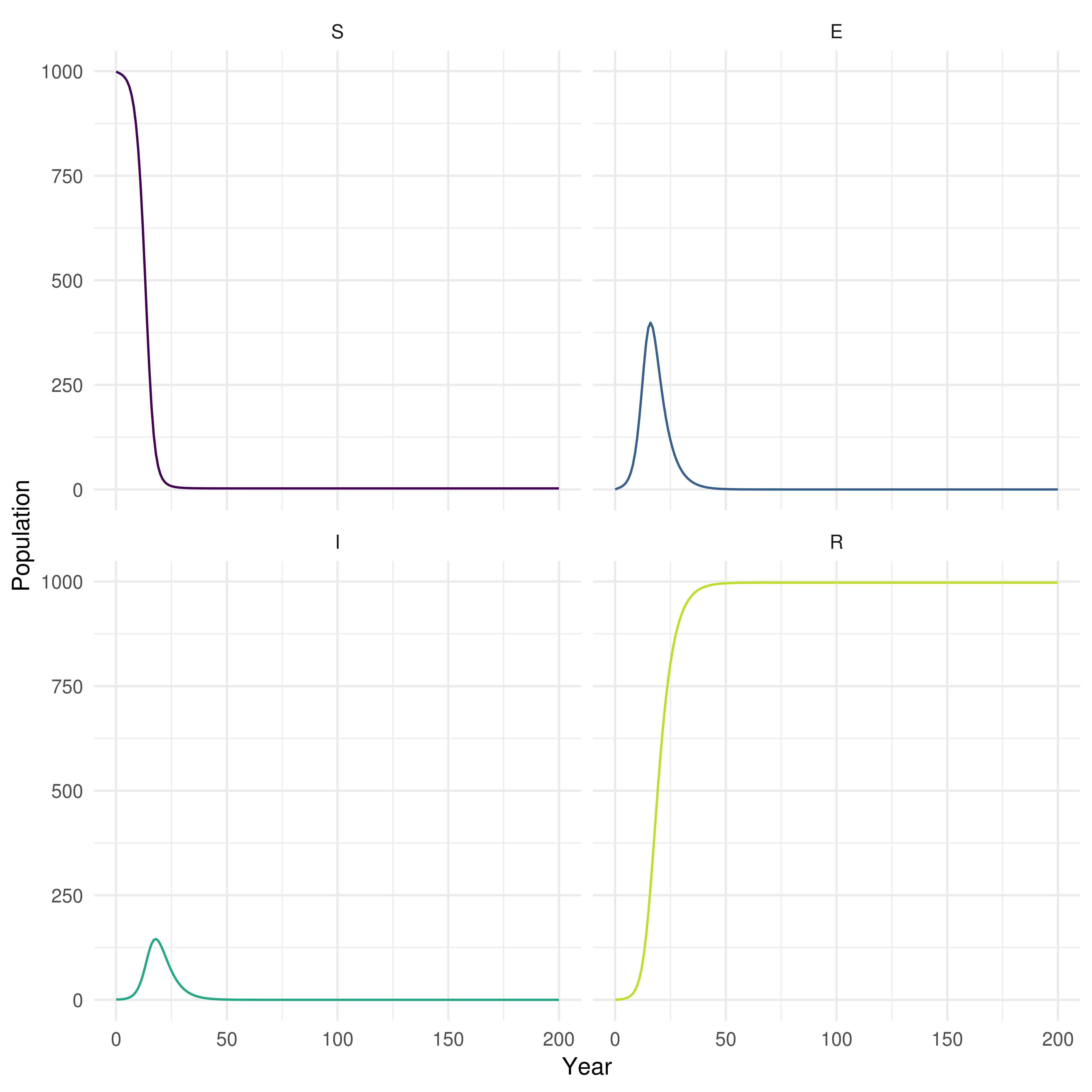

Figure 1: Plot of population over time in each SEIR model compartment

Explore

As we saw in practical 2, model dynamics are parameter dependent. Look back at the questions from practical 2 and check that you can implement the changes in the code above to answer them.

2. Add High and Low Risk Compartments

Now we are going to implement the SHLIR model from practical 2 and try to reproduce some of the behaviour observed using the interactive interface. See practical 2 for details on this model.

Populations and Initialisation

As in the previous model the first step is to define the model populations. There are now two new compartments, high risk latents (H), and low risk latents (L). These replace the original latent population (E) used in the SEIR model.

SHLIR_inits = c(
  S = 999,
  H = 0,
  L = 0,
  I = 1,
  R = 0
)

Parameters

We add two additional parameters for the rate of progression from high to low risk latents (nu) and the rate of progression from low risk latent to active disease (gamma_L).

SHLIR_parameters <- c(
  beta = 3, # Rate of transmission
  gamma_H = 1/5, # Rate of progression to active symptoms from high risk latent
  nu = 1/2, #Rate of progression from high to low risk latent
  gamma_L = 1/100, # Rate of progression to active symptoms for low risk latent
  tau = 1/2, # Rate of recovery
  mu = 1/81 # Rate of natural mortality
)

Equations

The code below is a starting point, fill in the missing model terms using the model flow diagram (Figure 2) and the code for the previous SEIR model as reference points.

SHLIR_demo_ode <- function(t, x, params) {

  ## Specify model compartments
  S <- x[1]
  H <- x[2]
  L <- x[3]
  I <- x[4]
  R <- x[5]

  with(as.list(params),{

    ## Specify total population
    N = S + H + L + I + R

    ## Derivative Expressions
    dS = - beta * S * I / N - mu * S + mu * N
    ## These are the new equations - fill in the remaining terms
    dH = beta * (S + L) * I / N - gamma_H * H - nu * H - mu * H
    dL = nu * H - beta * L * I / N - gamma_L * L - mu * L
    ## Hint terms are missing from this equation as well
    dI = gamma_H * H + gamma_L * L - tau * I - mu * I
    dR = tau * I - mu * R

    ## output
    derivatives <- c(dS, dH, dL, dI, dR)

    list(derivatives)
  })
}

Simulate and Summarise

Simulation is the same as for the previous model. Does the simulation of your improved model make sense? Evaluate the summary tables and plot of model populations over time.

begin_time <- 0
end_time <- 200
SHILR_times <- seq(begin_time, end_time, 1)

## see ?solve_ode for details
SHLIR_sim <- biddmodellingcourse::solve_ode(model = SHLIR_demo_ode, 
                                           inits = SHLIR_inits, 
                                           params = SHLIR_parameters,
                                           times = SHILR_times, 
                                           as.data.frame = TRUE)
SHLIR_sim %>% 
  head %>% 
  pretty_table(caption = "First 5 years of SHLIR model simulation",
               label = "tab-1")

Table 1: First 5 years of model simulation

time	S	H	L	I	R
0	999	0	0	1	0
1	996.5	1.794	0.5224	0.7773	0.4223
2	994.2	2.576	1.606	0.8263	0.8098
3	991.6	3.186	2.99	0.9684	1.243
4	988.6	3.853	4.648	1.164	1.756
5	984.9	4.653	6.621	1.411	2.372

biddmodellingcourse::summarise_model(SHLIR_sim) %>% 
  pretty_table(caption = "SHLIR model summary statistics; The final size of each population at the end of the simulation, along with the time the epidemic peak was reached, the number of infected at the epidemic peak and the duration of the epidemic")

Table 3: SHLIR model summary statistics; The final size of each population at the end of the simulation, along with the time the epidemic peak was reached, the number of infected at the epidemic peak and the duration of the epidemic (continued below)

Final size: S	Final size: H	Final size: L	Final size: I	Final size: R
238	24	194	13	531

Epidemic peak time	Epidemic peak	Epidemic duration
32	57	1

## For an interactive graph change interactive to TRUE
biddmodellingcourse::plot_model(SHLIR_sim, interactive = FALSE)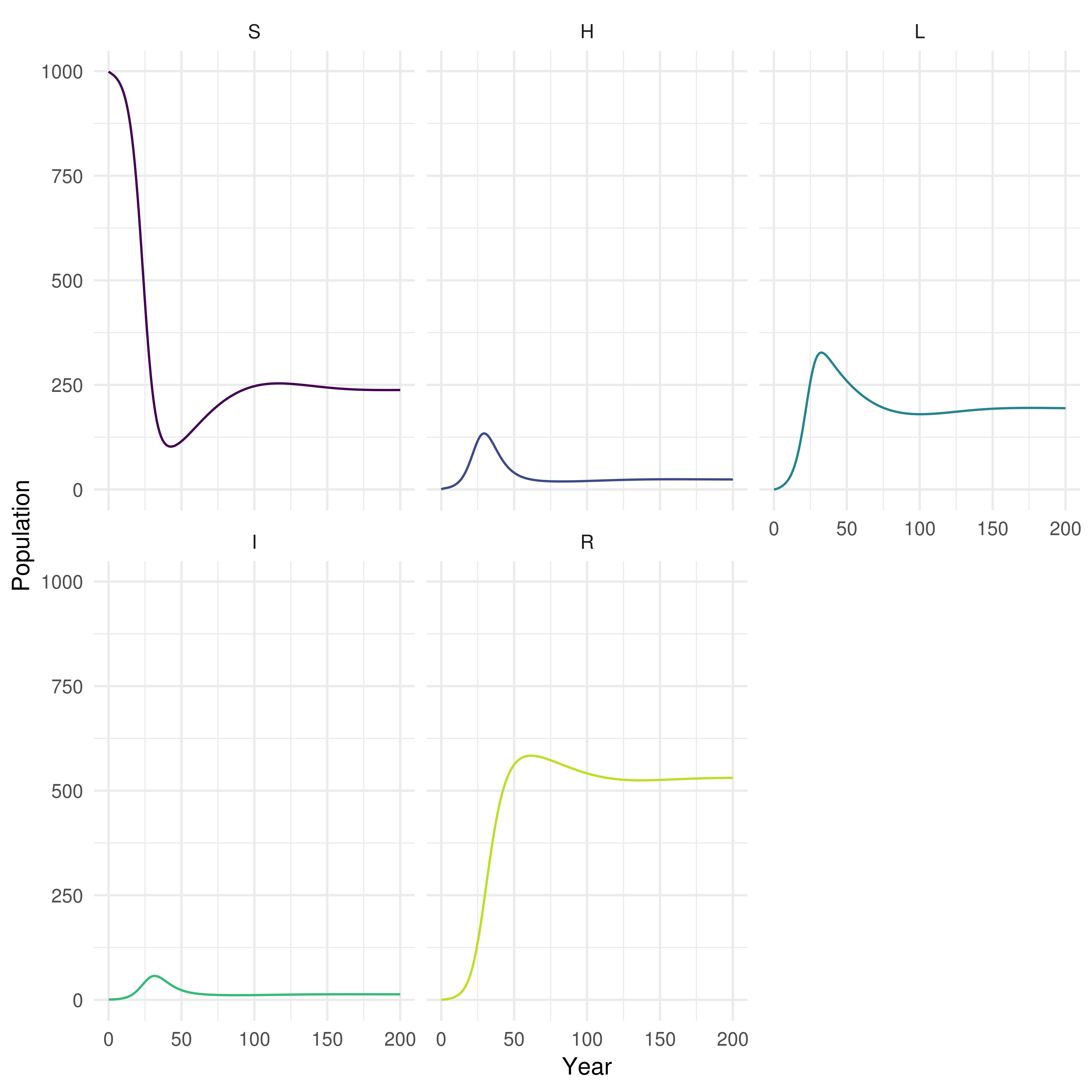

Figure 3: Plot of the population in each SHLIR model compartment over time

Explore

1. Test your changes by setting nu = 0 and all other parameters to be the same as for the SEIR model. If everything is working correctly both models should give the same output.

   • The SEIR and SHLIR models should give the same result.
   • This works because when nu = 0 no one enters the low risk latent population compartment and therefore it has no effect.

2. Can you alter the parameters defined above to answer the questions for the SHLIR model from practical 2?

3. Translate a more realistic SHLIR model flow diagram to equations

As a more advanced exercise (feel free to skip this if wanting to design your own model now) we now translate the more complex SHLIR model into code. Look back at practical 2 for a refresher on the structure of this model.

Populations and Initialisation

The new populations have been added for you. The population has now been split between low and high risk populations, with the only infectious case being in the high risk population.

real_SHLIR_inits = c(
  # General population
  S = 800,
  H = 0,
  L = 0,
  I = 0,
  Tr = 0,
  R = 0,
  ## High risk population
  S_H = 199,
  H_H = 0,
  L_H = 0,
  I_H = 1,
  Tr_H = 0,
  R_H = 0
)

Parameters

The required model parameters have been defined for you (with the units being years^-1). The only new parameters are the between group mixing (M), the proportion that are born high risk (p), and the transmission probability in those considered to be high risk (beta_H).

real_SHLIR_parameters <- c(
  beta = 3, # Rate of transmission
  beta_H = 6, # High risk rate of transmission
  gamma_H = 1/5, # Rate of progression to active symptoms from high risk latent
  nu = 1/2, #Rate of progression from high to low risk latent
  gamma_L = 1/100, # Rate of progression to active symptoms for low risk latent
  epsilon = 1/3, # Rate of treatment
  tau = 1/2, # Rate of recovery
  mu = 1/81, # Rate of natural mortality
  p = 0.2, # proportion of new births that are high risk
  M = 0.2 # Between group mixing
)

Equations

Update the model equations using the model flow diagram above. The comments in the code given hints as to where changes need to be made. The equations for the low risk population have been provided for you.

real_SHLIR_demo_ode <- function(t, x, params) {

  ## Specify model compartments 
  ## The compartments for the low risk population have been provided 
  ## Add the high risk population
  ## Don't forget to update indexing for x. Compare the previous two models for a hint.
  S <- x[1]
  H <- x[2]
  L <- x[3]
  I <- x[4]
  Tr <- x[5]
  R <- x[6]
  
  S_H <- x[7]
  H_H <- x[8]
  L_H <- x[9]
  I_H <- x[10]
  Tr_H <- x[11]
  R_H <- x[12]

  with(as.list(params),{

    ## Specify total population
    N = S + H + L + I + Tr + R + S_H + H_H + L_H + I_H + Tr_H + R_H

    ## Force of infection
    ## The force of infetion in the low risk population has been provided for you
    foi <- beta  * I / N + M * beta_H * I_H / N 
    ## Add the high risk force of infection here
    foi_H <-  M * beta  * I / N +  beta_H * I_H / N 
    
    ## Derivative Expressions
    ## General population - provided for you
    ## Compare these equations from those used for the previous models
    dS = -S * foi - mu * S + (1 - p) * mu * N
    dH = (S + L + R) * foi - gamma_H * H - nu * H - mu * H
    dL = nu * H - L * foi - gamma_L * L - mu * L
    dI = gamma_H * H + gamma_L * L - epsilon * I - mu * I
    dTr = epsilon * I - tau * Tr - mu * Tr
    dR = tau * Tr - R * foi - mu * R
    
    ## High risk population
    ## Copy the equations used above for the low risk population
    ## Convert them to be in the high risk population
    dS_H = -S_H * foi_H - mu * S_H + p * mu * N
    dH_H = (S_H + L_H + R_H) * foi_H - gamma_H * H_H - nu * H_H - mu * H_H
    dL_H = nu * H_H - L_H * foi_H - gamma_L * L_H - mu * L_H
    dI_H = gamma_H * H_H + gamma_L * L_H - epsilon * I_H - mu * I_H
    dTr_H = epsilon * I_H - tau * Tr_H - mu * Tr_H
    dR_H = tau * Tr_H - R_H * foi_H - mu * R_H

    ## output
    derivatives <- c(dS, dH, dL, dI, dTr, dR, dS_H, dH_H, dL_H, dI_H, dTr_H, dR_H)

    list(derivatives)
  })
}

Simulate and Summarise

Simulate the new model as previously.

begin_time <- 0
end_time <- 200
real_SHLIR_times <- seq(begin_time, end_time, 1)

## see ?solve_ode for details
real_SHLIR_sim <- biddmodellingcourse::solve_ode(model = real_SHLIR_demo_ode, 
                                           inits = real_SHLIR_inits, 
                                           params = real_SHLIR_parameters,
                                           times = real_SHLIR_times, 
                                           as.data.frame = TRUE)
real_SHLIR_sim %>% 
  head %>% 
  pretty_table(caption = "First 5 years of model simulation",
               label = "tab-real_SHLIR")

Table 4: First 5 years of model simulation (continued below)

time	S	H	L	I	Tr	R	S_H
0	800	0	0	0	0	0	199
1	799.1	0.6388	0.1786	0.06452	0.006904	0.0009364	198
2	798.1	1.048	0.5935	0.1941	0.03844	0.01108	197.1
3	796.8	1.477	1.201	0.3596	0.09632	0.04336	196.3
4	795.1	2.002	2.027	0.5632	0.1794	0.1102	195.5
5	792.9	2.658	3.121	0.8155	0.2889	0.2236	194.6

H_H	L_H	I_H	Tr_H	R_H
0	0	1	0	0
0.7367	0.2138	0.785	0.2257	0.06372
0.9991	0.6472	0.7108	0.3277	0.2031
1.106	1.153	0.6904	0.3781	0.3761
1.169	1.684	0.6935	0.4067	0.565
1.228	2.23	0.7103	0.4267	0.7623

biddmodellingcourse::summarise_model(real_SHLIR_sim) %>% 
  pretty_table(caption = "Realistic SHLIR model summary statistics; The final size of each population at the end of the simulation, along with the time the epidemic peak was reached, the number of infected at the epidemic peak and the duration of the epidemic")

Table 5: Realistic SHLIR model summary statistics; The final size of each population at the end of the simulation, along with the time the epidemic peak was reached, the number of infected at the epidemic peak and the duration of the epidemic (continued below)

Final size: S	Final size: H	Final size: L	Final size: I	Final size: Tr
22	218	242	133	87

Table continues below

Final size: R	Final size: S_H	Final size: H_H	Final size: L_H
98	10	39	77

Table continues below

Final size: I_H	Final size: Tr_H	Final size: R_H	Epidemic peak time
25	16	33	74

Epidemic peak	Epidemic duration
133	0

## For an interactive graph change interactive to TRUE
biddmodellingcourse::plot_model(real_SHLIR_sim, interactive = FALSE)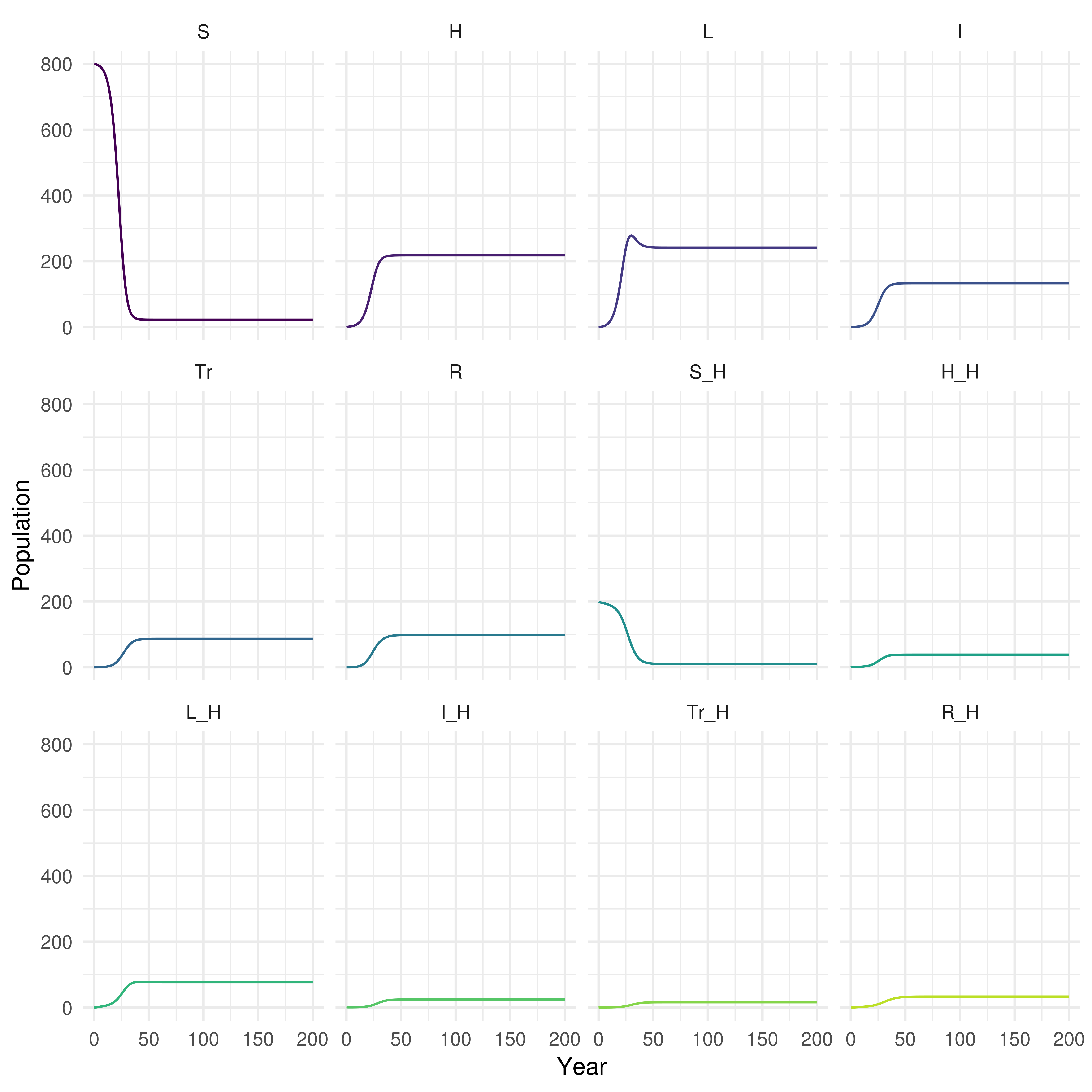

Figure 4: Plot of population over time in each realistic SHLIR model compartment

Explore

1. Test your changes by setting all the parameters to be the same as in the SHLIR model.

   • The models should give the same results.

2. Can you alter the parameters defined above to answer the questions for this model from practical 2?

4. Implement Your Own Model

Using the same structure as used in models above implement your own model into R. Talk to the instructors for tips, tricks, and potential ideas. See the idmodelr package for other example model structures (https://www.samabbott.co.uk/idmodelr/). It may help to first draw out the flow diagram for your model (potentially writing out the equations may also help).