Practical 2: Exploring Compartmental Model Dynamics
Sam Abbott
Source:vignettes/practical-two.Rmd
practical-two.RmdLearning Objectives
- Understand how changing parameter values, and model structure, can influence model dynamics.
- Understand the dynamics of the SEIR model in detail.
- Understand the impact of risk group stratification on model dynamics.
- Understand some of the complex dynamics produced by a more realistic model.
Outline for Session
- Set up (5 minutes)
- Investigate the dynamics of a simple SEIR model (20 minutes)
- Explore the impact of adding high and low risk latency to a SEIR model, in comparison to the SEIR model (10 minutes).
- Investigate the complex dynamics of a more realistic SHLIR model (10 minutes) .
- Explore the parameter space of multiple models and try to understand some of the general implications of model structures on dynamics (10 minutes).
- Session wrap up (5 minutes)
Set up
In order to more systematically explore the parameter space of multiple models we have provided an interactive interface. Start the interactive interface by running the following in R.
if (!library(shiny, logical.return = TRUE)) {
  install.packages("shiny")
  library(shiny)
}
shiny::runGitHub("exploreidmodels", "seabbs")
If having problems running the application then talk to an instructor and/or try the hosted web version (http://seabbs.co.uk/shiny/exploreidmodels/).
Use this interface to explore the some of the model that have already been discussed and to answer the following ec. Instructions for using the interactive interface can be found in the about section of the application.
Exercises
1. A Simple SEIR Model of Tuberculosis (TB)
As a first exercise, we are going to explore the simple SEIR model (select it in the interface), as seen in the design a model practical. For reference the SEIR model flow diagram seen in the first practical’s solutions.[1] The equations below are a translation of this into R code.
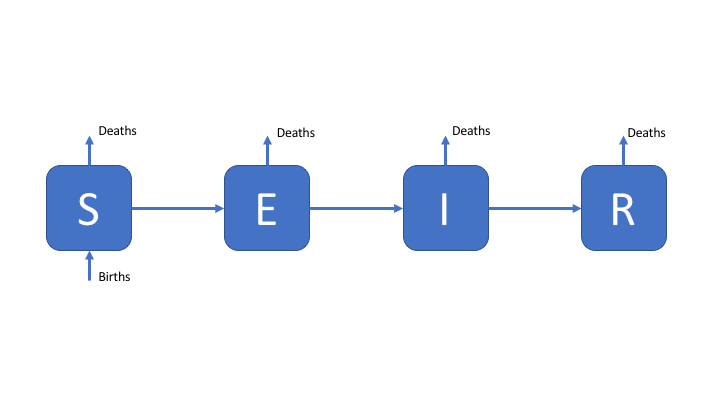
Figure 1: An SEIR model of TB transmission, including simple demographic processes
Explore
Model dynamics are parameter dependent. Even in a simplistic model like the one outlined above parameter values can greatly alter the dynamics. Answer the following questions by varying the parameters and rerunning the model.
Set a transmission rate (beta) of 7, an infectios period of 3 months, and a latent period of 0. What role does the latent period have with these settings? What happens to the number of susceptibles over time?
Increase the transmission rate and rerun the model. How does this impact the number of infected individuals?
Increase the infectious period. How does a longer infectious period impact the shape of the epidemic curve?
Increase the latent period to 6 months. What impacts does this have on the disease outbreak?
Set beta to 3, the infectious period 12 months, the latent period to 0, and set the timespan to 100. Run the model, turn on demographic processes, and then re-run the model. What is the impact of adding demographic processes (births and deaths)?
Reduce the life expectancy to 20 years. What impact does this have on the infected population?
2. Add High and Low Risk Compartments
To make the SEIR model slightly more realistic, and therefore better able to capture the observed dynamics of TB, we add a second latent population (as discussed in the solutions for practical 1). This change can be seen in the model flow diagram (Figure 2). Go back to practical 1 if you need a refresher for the motivation behind this. We have also added reinfection for the low risk latent population.
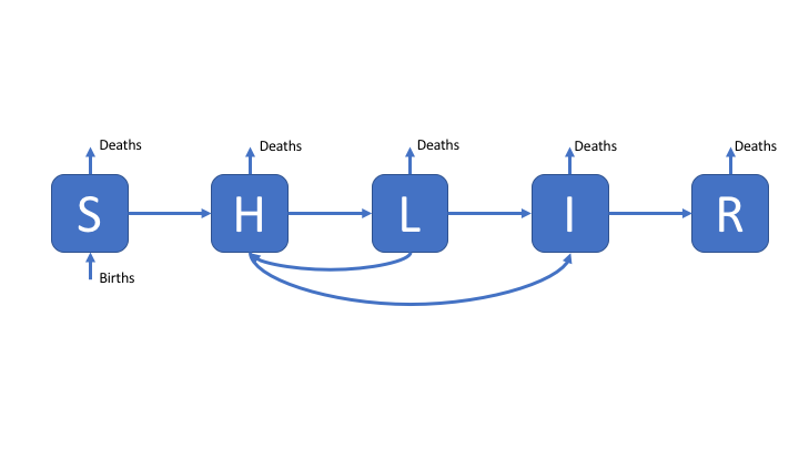
Figure 2: An SHLIR model of TB transmission, including simple demographic processes
Explore
Switch to the SHLIR model and turn off demographic processes. Set beta to 9, the high risk latent period to 0, the low risk period to 20 years, the infectious period to 12 months, and the timespan to 100 years. Run this model (this is effectively the SEIR model, see the flow diagram to understand why). Now set the high risk latent period to 2 years, and the rate of developing active disease when high risk to 0.6 - re-run the model. What is the impact of the second high risk latent compartment?
Re-run the model with demographic processes (with a life expectancy of 20 years). What impact do they have on the dynamics?
3. A more realistic SHLIR model flow diagram
The most complex model supported by the interactive interface, this is a more realistic model that might be used in research. The SHLIR model flow diagram (Figure 3) includes: risk groups, treatment, and reinfection for those who have recovered from active disease. Whilst many realistic TB models use age structure this is not included here (if you are interested in discussing how you would include this talk to your instructors or contact me). For simplicity we have assumed that it is possible to be born into both populations. For the motivation behind this model see practical 1.
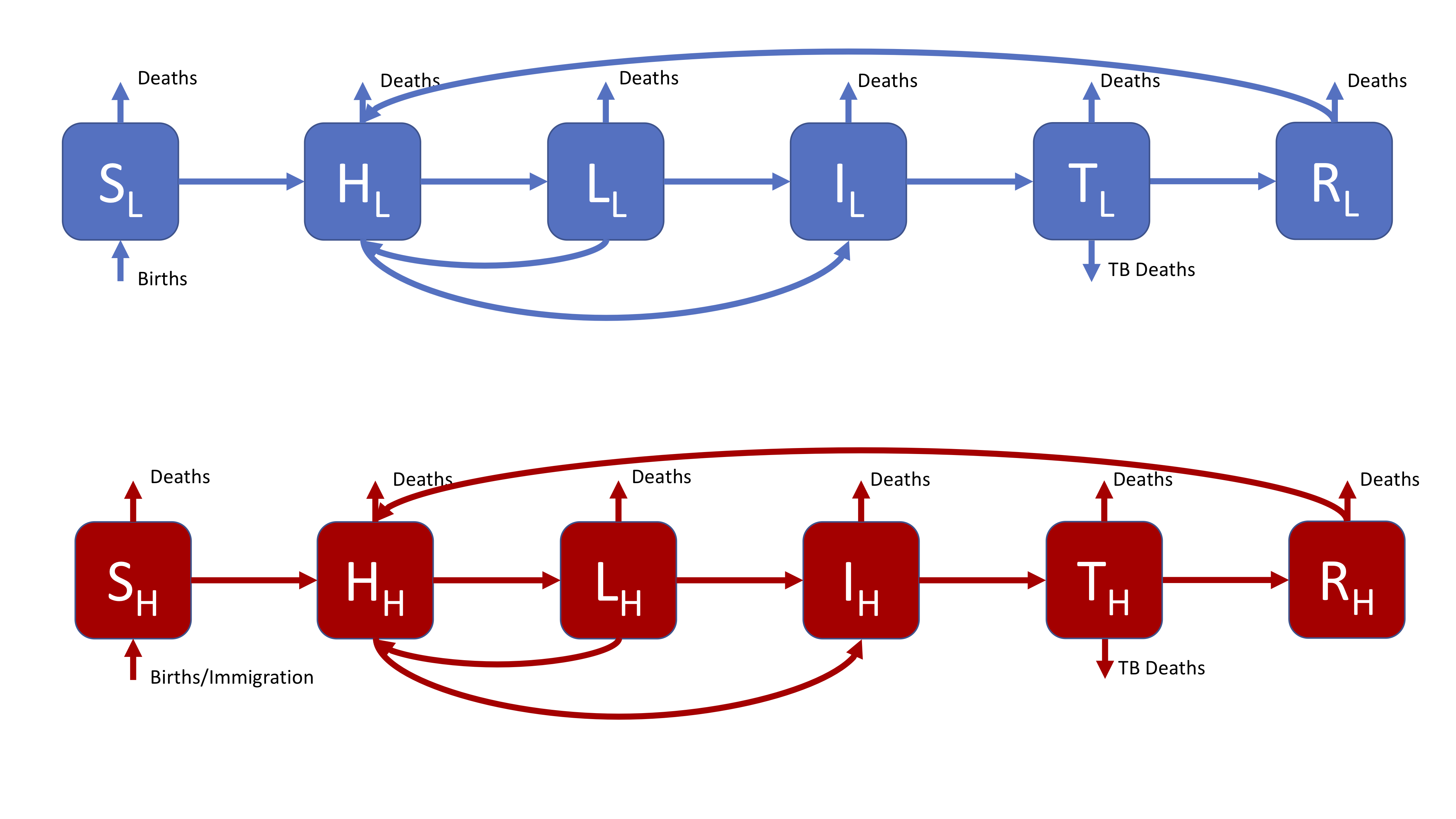
Figure 3: A realistic SHLIR model of TB transmission, including simple demographic processes
Figure 3 does not include the interaction between the high and low risk subgroups as this is through the force of infection. The force of infection is defined as,
\[ \lambda_i = \beta \sum_{j = L, H}M_{ij}I_j \]
Where \(\lambda_i\) is the force of infection in each risk group (\(i = L, H\)) and \(M_{LH}\) is the mixing rate between risk groups. It is assumed that within group contact rates are equivalent and defined such that,
\[ M_{ii} = 1 \]
It is also assumed that the between group contact rates are defined as (where \(i \neq j\)),
\[ M_{ij} = 0.1 \]
Explore
Select the SHLITR model with risk groups. Run it with a beta of 3, a high risk beta of 3, a life expectancy of 1000, and all other parameters as set. Re-run the model with a high risk beta of 30. What is the impact of the high risk group on the number of cases?
Set beta to be 0.5, the between group mixing to be 0 and run the model. Now set the between group mixing to be 0.2 and re-run the model. With these parameter settings what differences do you see between these model runs? Can you explain these findings (see the model outline above for hints)?
What is the impact of varying the mixing between high and low risk groups for the above scenario?
References
1 Brooks-Pollock E, Cohen T, Murray M. The impact of realistic age structure in simple models of tuberculosis transmission. PLoS One 2010;5:3–8. doi:10.1371/journal.pone.0008479